Maximum penalized likelihood estimation of a Generalized Additive model for the copula parameter or Kendall's tau.

This function estimates the parameter(s) of a Generalized Additive model (gam) for the copula parameter or Kendall's tau. It solves the maximum penalized likelihood estimation for the copula families supported in this package by reformulating each Newton-Raphson iteration as a generalized ridge regression, which is solved using the mgcv package.

gamBiCopFit(
  data,
  formula = ~1,
  family = 1,
  tau = TRUE,
  method = "FS",
  tol.rel = 0.001,
  n.iters = 10,
  verbose = FALSE,
  ...
)

Arguments

data: A list, data frame or matrix containing the model responses, (u1,u2) in [0,1]x[0,1], and covariates required by the formula.
formula: A gam formula (see gam, formula.gam and gam.models from mgcv).
family: A copula family: 1 Gaussian, 2 Student t, 5 Frank, 301 Double Clayton type I (standard and rotated 90 degrees), 302 Double Clayton type II (standard and rotated 270 degrees), 303 Double Clayton type III (survival and rotated 90 degrees), 304 Double Clayton type IV (survival and rotated 270 degrees), 401 Double Gumbel type I (standard and rotated 90 degrees), 402 Double Gumbel type II (standard and rotated 270 degrees), 403 Double Gumbel type III (survival and rotated 90 degrees), 404 Double Gumbel type IV (survival and rotated 270 degrees).
tau: FALSE (default) for a calibration function specified for the Copula parameter or TRUE for a calibration function specified for Kendall's tau.
method: 'NR' for Newton-Raphson and 'FS' for Fisher-scoring (default).
tol.rel: Relative tolerance for 'FS'/'NR' algorithm.
n.iters: Maximal number of iterations for 'FS'/'NR' algorithm.
verbose: TRUE if informations should be printed during the estimation and FALSE (default) for a silent version.
...: Additional parameters to be passed to gam from mgcv.

Value

gamBiCopFit returns a list consisting of

res: S4 gamBiCop-class object.
method: 'FS' for Fisher-scoring (default) and 'NR' for Newton-Raphson.
tol.rel: relative tolerance for 'FS'/'NR' algorithm.
n.iters: maximal number of iterations for 'FS'/'NR' algorithm.
trace: the estimation procedure's trace.
conv: 0 if the algorithm converged and 1 otherwise.

Examples

require(copula)
require(mgcv)
#> Loading required package: mgcv
#> Loading required package: nlme
#> This is mgcv 1.9-1. For overview type 'help("mgcv-package")'.
set.seed(0)

## Simulation parameters (sample size, correlation between covariates,
## Gaussian copula family)
n <- 5e2
rho <- 0.5
fam <- 1


## A calibration surface depending on three variables
eta0 <- 1
calib.surf <- list(
  calib.quad <- function(t, Ti = 0, Tf = 1, b = 8) {
    Tm <- (Tf - Ti) / 2
    a <- -(b / 3) * (Tf^2 - 3 * Tf * Tm + 3 * Tm^2)
    return(a + b * (t - Tm)^2)
  },
  calib.sin <- function(t, Ti = 0, Tf = 1, b = 1, f = 1) {
    a <- b * (1 - 2 * Tf * pi / (f * Tf * pi +
      cos(2 * f * pi * (Tf - Ti))
      - cos(2 * f * pi * Ti)))
    return((a + b) / 2 + (b - a) * sin(2 * f * pi * (t - Ti)) / 2)
  },
  calib.exp <- function(t, Ti = 0, Tf = 1, b = 2, s = Tf / 8) {
    Tm <- (Tf - Ti) / 2
    a <- (b * s * sqrt(2 * pi) / Tf) * (pnorm(0, Tm, s) - pnorm(Tf, Tm, s))
    return(a + b * exp(-(t - Tm)^2 / (2 * s^2)))
  }
)

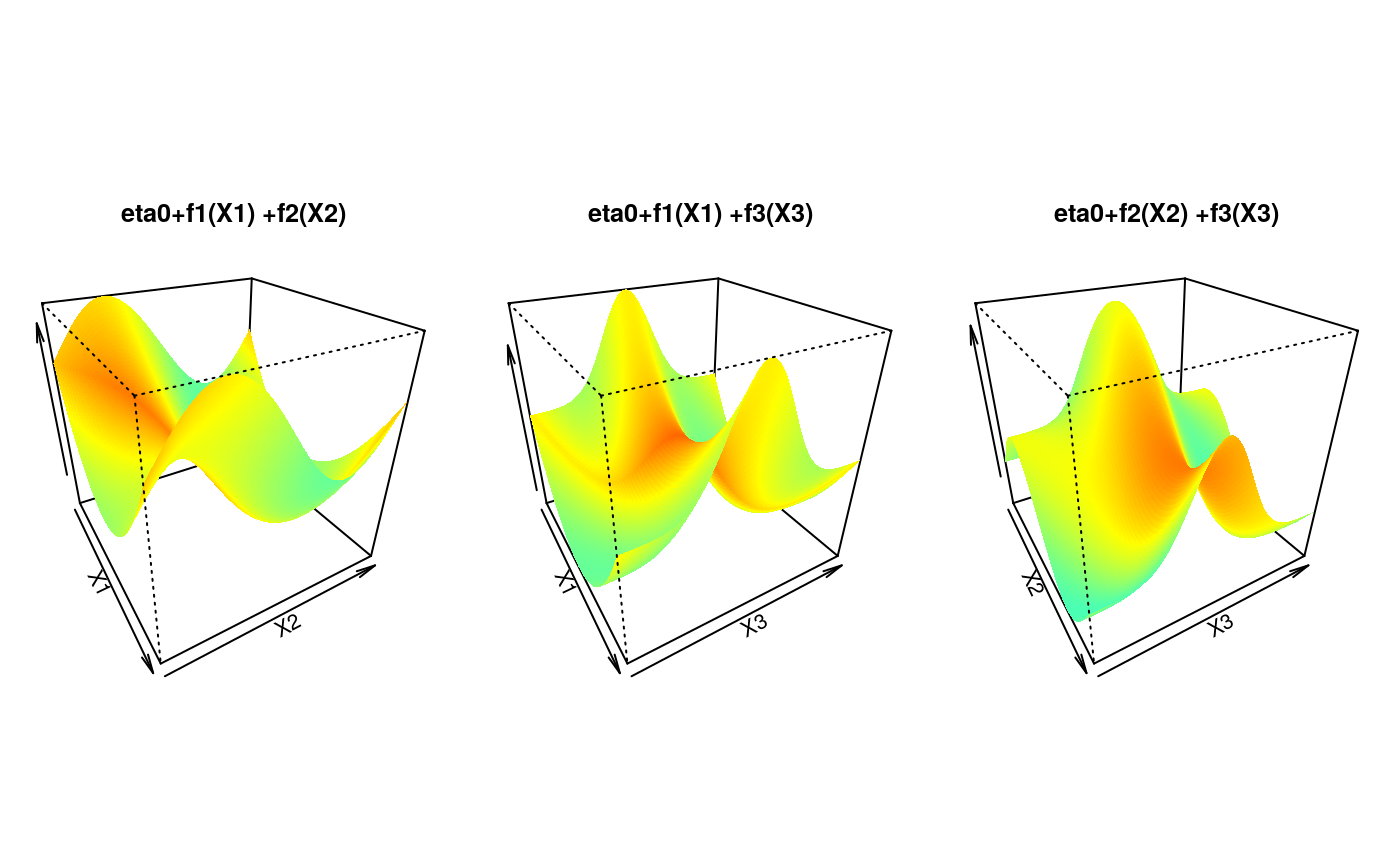
## Display the calibration surface
par(mfrow = c(1, 3), pty = "s", mar = c(1, 1, 4, 1))
u <- seq(0, 1, length.out = 100)
sel <- matrix(c(1, 1, 2, 2, 3, 3), ncol = 2)
jet.colors <- colorRamp(c(
  "#00007F", "blue", "#007FFF", "cyan", "#7FFF7F",
  "yellow", "#FF7F00", "red", "#7F0000"
))
jet <- function(x) rgb(jet.colors(exp(x / 3) / (1 + exp(x / 3))),
    maxColorValue = 255
  )
for (k in 1:3) {
  tmp <- outer(u, u, function(x, y)
    eta0 + calib.surf[[sel[k, 1]]](x) + calib.surf[[sel[k, 2]]](y))
  persp(u, u, tmp,
    border = NA, theta = 60, phi = 30, zlab = "",
    col = matrix(jet(tmp), nrow = 100),
    xlab = paste("X", sel[k, 1], sep = ""),
    ylab = paste("X", sel[k, 2], sep = ""),
    main = paste("eta0+f", sel[k, 1],
      "(X", sel[k, 1], ") +f", sel[k, 2],
      "(X", sel[k, 2], ")",
      sep = ""
    )
  )
}


## 3-dimensional matrix X of covariates
covariates.distr <- mvdc(normalCopula(rho, dim = 3),
  c("unif"), list(list(min = 0, max = 1)),
  marginsIdentical = TRUE
)
X <- rMvdc(n, covariates.distr)

## U in [0,1]x[0,1] with copula parameter depending on X
U <- condBiCopSim(fam, function(x1, x2, x3) {
  eta0 + sum(mapply(function(f, x)
    f(x), calib.surf, c(x1, x2, x3)))
}, X[, 1:3], par2 = 6, return.par = TRUE)

## Merge U and X
data <- data.frame(U$data, X)
names(data) <- c(paste("u", 1:2, sep = ""), paste("x", 1:3, sep = ""))

## Display the data
dev.off()
#> null device 
#>           1 
plot(data[, "u1"], data[, "u2"], xlab = "U1", ylab = "U2")

## Model fit with a basis size (arguably) too small
## and unpenalized cubic spines
pen <- FALSE
basis0 <- c(3, 4, 4)
formula <- ~ s(x1, k = basis0[1], bs = "cr", fx = !pen) +
  s(x2, k = basis0[2], bs = "cr", fx = !pen) +
  s(x3, k = basis0[3], bs = "cr", fx = !pen)
system.time(fit0 <- gamBiCopFit(data, formula, fam))
#>    user  system elapsed 
#>   0.097   0.001   0.098 

## Model fit with a better basis size and penalized cubic splines (via min GCV)
pen <- TRUE
basis1 <- c(3, 10, 10)
formula <- ~ s(x1, k = basis1[1], bs = "cr", fx = !pen) +
  s(x2, k = basis1[2], bs = "cr", fx = !pen) +
  s(x3, k = basis1[3], bs = "cr", fx = !pen)
system.time(fit1 <- gamBiCopFit(data, formula, fam))
#>    user  system elapsed 
#>   0.479   1.568   0.338 

## Extract the gamBiCop objects and show various methods
(res <- sapply(list(fit0, fit1), function(fit) {
  fit$res
}))
#> [[1]]
#> Gaussian copula with tau(z) = (exp(z)-1)/(exp(z)+1) where 
#> z ~ s(x1, k = basis0[1], bs = "cr", fx = !pen) + s(x2, k = basis0[2], 
#>     bs = "cr", fx = !pen) + s(x3, k = basis0[3], bs = "cr", fx = !pen)
#> 
#> [[2]]
#> Gaussian copula with tau(z) = (exp(z)-1)/(exp(z)+1) where 
#> z ~ s(x1, k = basis1[1], bs = "cr", fx = !pen) + s(x2, k = basis1[2], 
#>     bs = "cr", fx = !pen) + s(x3, k = basis1[3], bs = "cr", fx = !pen)
#> 
metds <- list("logLik" = logLik, "AIC" = AIC, "BIC" = BIC, "EDF" = EDF)
lapply(res, function(x) sapply(metds, function(f) f(x)))
#> [[1]]
#> [[1]]$logLik
#> 'log Lik.' 266.8974 (df=9)
#> 
#> [[1]]$AIC
#> [1] -515.7948
#> 
#> [[1]]$BIC
#> [1] -477.8633
#> 
#> [[1]]$EDF
#> [1] 1 2 3 3
#> 
#> 
#> [[2]]
#> [[2]]$logLik
#> 'log Lik.' 302.9581 (df=16.24202)
#> 
#> [[2]]$AIC
#> [1] -573.4321
#> 
#> [[2]]$BIC
#> [1] -504.9783
#> 
#> [[2]]$EDF
#> [1] 1.000000 1.999178 7.577543 5.665301
#> 
#> 


## Comparison between fitted, true smooth and spline approximation for each
## true smooth function for the two basis sizes
fitted <- lapply(res, function(x) gamBiCopPredict(x, data.frame(x1 = u, x2 = u, x3 = u),
    type = "terms"
  )$calib)
true <- vector("list", 3)
for (i in 1:3) {
  y <- eta0 + calib.surf[[i]](u)
  true[[i]]$true <- y - eta0
  temp <- gam(y ~ s(u, k = basis0[i], bs = "cr", fx = TRUE))
  true[[i]]$approx <- predict.gam(temp, type = "terms")
  temp <- gam(y ~ s(u, k = basis1[i], bs = "cr", fx = FALSE))
  true[[i]]$approx2 <- predict.gam(temp, type = "terms")
}

## Display results
par(mfrow = c(1, 3), pty = "s")
yy <- range(true, fitted)
yy[1] <- yy[1] * 1.5
for (k in 1:3) {
  plot(u, true[[k]]$true,
    type = "l", ylim = yy,
    xlab = paste("Covariate", k), ylab = paste("Smooth", k)
  )
  lines(u, true[[k]]$approx, col = "red", lty = 2)
  lines(u, fitted[[1]][, k], col = "red")
  lines(u, fitted[[2]][, k], col = "green")
  lines(u, true[[k]]$approx2, col = "green", lty = 2)
  legend("bottomleft",
    cex = 0.6, lty = c(1, 1, 2, 1, 2),
    c("True", "Fitted", "Appox 1", "Fitted 2", "Approx 2"),
    col = c("black", "red", "red", "green", "green")
  )
}

Maximum penalized likelihood estimation of a Generalized Additive model for the copula parameter or Kendall's tau.

Arguments

Value

See also

Examples